This is part 2/8 of my Calculating Percentiles on Streaming Data series.
The most famous algorithm for calculating percentiles on streaming data appears to be Greenwald-Khanna [GK01]. I spent a few days implementing the Greenwald-Khanna algorithm from the paper and I discovered a few things I wanted to share.
Insert Operation
The insert operation is defined in [GK01] as follows:
- INSERT($v$)
- Find the smallest $i$, such that $v_{i-1} \leq v < v_i$, and insert the tuple $ t_x = (v_x, g_x, \Delta_x) = (v, 1, \lfloor 2 \epsilon n \rfloor) $, between $t_{i-1}$ and $t_i$. Increment $s$. As a special case, if $v$ is the new minimum or the maximum observation seen, then insert $(v, 1, 0)$.
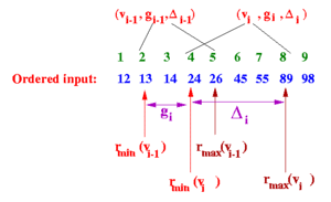
However, when I implemented this operation, I noticed via testing that there were certain queries I could not fulfill. For example, consider applying Greenwald-Khanna with $\epsilon = 0.1$ to the sequence of values ${11, 20, 18, 5, 12, 6, 3, 2}$, and then apply QUANTILE($\phi = 0.5$). This means that $r = \lceil \phi n \rceil = \lceil 0.5 \times 8 \rceil = 4$ and $\epsilon n = 0.1 \times 8 = 0.8$. There is no $i$ that satisfies both $r – r_{min}(v_i) \leq \epsilon n$ and $r_{max}(v_i) – r \leq \epsilon n$, as you can see below:
| $i$ | $t_i$ | $r_{min}$ | $r_{max}$ | $r – r_{min}$ | $r_{max}-r$ | $r – r_{min}\overset{?}{\leq}\epsilon n$ | $r_{max} – r\overset{?}{\leq}\epsilon n$ |
|---|---|---|---|---|---|---|---|
| (2,1,0) | 1 | 1 | 3 | -3 | F | T | |
| 1 | (3,1,0) | 2 | 2 | 2 | -2 | F | T |
| 2 | (5,1,0) | 3 | 3 | 1 | -1 | F | T |
| 3 | (6,1,1) | 4 | 5 | 0 | 1 | T | F |
| 4 | (11,1,0) | 5 | 5 | -1 | 1 | T | F |
| 5 | (12,1,0) | 6 | 6 | -2 | 2 | T | F |
| 6 | (18,1,0) | 7 | 7 | -3 | 3 | T | F |
| 7 | (20,1,0) | 8 | 8 | -4 | 4 | T | F |
I believe the fundamental problem is that the definition of INSERT($v$) fails to maintain the key invariant $\textrm{max}_i(g_i + \Delta_i) \leq 2 \epsilon n$. To correct this issue, the Greenwald-Khanna INSERT($v$) operation must be modified as follows:
- INSERT($v$)*
- Find the smallest $i$, such that $v_{i-1} \leq v < v_i$, and insert the tuple $t_x = (v_x, g_x, \Delta_x) = (v, 1, \lfloor 2 \epsilon n \rfloor – 1)$, between $t_{i-1}$ and $t_i$. Increment $s$. As a special case, if $v$ is the new minimum or the maximum observation seen, then insert $(v, 1, 0)$. Also, the first $1/(2 \epsilon)$ elements must be inserted with $\Delta_i = 0$.
I found the above modification from Prof. Chandra Chekuri’s lecture notes for his class CS 598CSC: Algorithms for Big Data. I believe this modification will maintain the above invariant after $1/(2 \epsilon) $ insertions.
Band Construction
Banding in [GK01] refers to the grouping together of possible values of $\Delta$ for purposes of merging in the COMPRESS operation. The paper defines banding as the following:
- BAND($\Delta$, $2 \epsilon n$)
- For $\alpha$ from 1 to $\lceil \log 2 \epsilon n \rceil$, we let $p = \lfloor 2 \epsilon n \rfloor$ and we define $\mathrm{band}_\alpha$ to be the set of all $\Delta$ such that $p – 2^\alpha – (p \mod 2^\alpha) < \Delta \leq p – 2^{\alpha – 1} – (p \mod 2^{\alpha – 1})$. We define $\mathrm{band}_{0}$ to simply be $p$. As a special case, we consider the first $1/2\epsilon$ observations, with $\Delta$ = 0, to be in a band of their own. We will denote by $\mathrm{band}(t_i, n)$ the band of $\Delta_i$ at time $n$, and by $\mathrm{band}_\alpha(n)$ all tuples (or equivalently, the $\Delta$ values associated with these tuples) that have a band value of $\alpha$.
Here are some things I found when implementing banding:
- It is important to note that in the above $\log$ refers to the base 2 logarithm of a number.
- I found it useful to construct an array, bands, at the beginning of the COMPRESS operation, such that bands[$\Delta$] is the band for the provided $\Delta$.
- I used a very large constant to denote the band of $\Delta = 0$, as this made the tree-building operation simpler.
Compress
Compression in [GK01] is defined as follows:
- COMPRESS()
- for $i$ from $s – 2$ to $0$ do …
However, with this definition, it is possible for the first (0th) tuple to be deleted, which would then violate the following invariant of the summary data structure: “We ensure that, at all times, the maximum and the minimum values are part of the summary.”
Therefore, I modified COMPRESS() to go from $s – 2$ to $1$ so that the first tuple is never deleted and the invariant is maintained.
References
- [GK01] M. Greenwald and S. Khanna. Space-efficient online computation of quantile summaries. In Proceedings of ACM SIGMOD, pages 58–66, 2001.