This is part 7/8 of my Calculating Percentiles on Streaming Data series.

In 2005, Graham Cormode, Flip Korn, S. Muthukrishnan, and Divesh Srivastava published a paper called Effective Computation of Biased Quantiles over Data Streams [CKMS05]. This paper took the Greenwald-Khanna algorithm [GK01] and made the following notable changes:

1. Generalized the algorithm to work with arbitrary targeted quantiles, where a targeted quantile is a combination of a quantile $\phi$ and a maximum allowable error $\epsilon$. The algorithm will maintain the summary data structure $\mathsf{S}$ such that it will maintain each targeted quantile with the appropriate error rate.
2. Simplified the Compress() operation by removing the concept of banding.

The paper also demonstrated that the new, more generalized algorithm could handle the following cases with ease:

1. The uniform quantile case, where each quantile is maintained with identical allowable error $\epsilon$.
2. The low-biased quantile case, where lower quantiles (i.e. as $\phi$ approaches 0) are maintained with higher precision (lower maximum allowable error) than higher quantiles.
3. The high-biased quantile case, where higher quantiles (i.e. as $\phi$ approaches 1) are maintained with higher precision (lower maximum allowable error) than lower quantiles.

Visualizing the Behavior of CKMS

Similar to my post about Visualizing Greenwald-Khanna, let’s visualize the above three cases with CKMS with $\epsilon = 0.1$.

Uniform Quantiles

Low-Biased Quantiles

High-Biased Quantiles

It’s quite visually intuitive how the low-biased quantiles case keeps more, finer-grained measurements at low percentile values, and the high-biased quantiles case keeps more, finer-grained measurements at high percentile values.

Understanding the CKMS Algorithm

Much of the below will only make sense if you have read the paper, so I suggest trying to read [CKMS05] first, and then returning here.

The key to understanding the CKMS algorithm is understanding the invariant function $f(r_i, n)$. I found that the best way to understand $f(r_i, n)$ is to understand the targeted quantiles invariant function (Definition 5 in [CKMS05]) and the error function $f(\phi n, n) / n$ charts (Figure 2 in [CKMS05]).

Uniform Quantiles Invariant Function

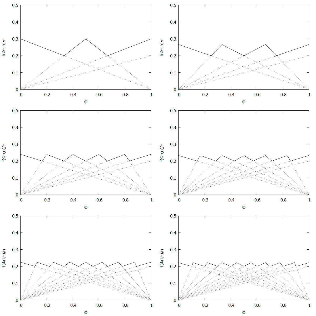
Consider the uniform quantile case, where we want all quantiles to be maintained with identical allowable error $\epsilon$. In this case, the targeted quantile tuples set will become $\mathsf{T} = {(\frac{1}{n}, \epsilon), (\frac{2}{n}, \epsilon), \ldots, (\frac{n-1}{n}, \epsilon), (1, \epsilon)}$.

Given the above definition, below is a visualization of the error function $f(\phi n)/n)$ computed for $\epsilon$ = 0.1 as $n$ increases from 3 to 10:

Visually, the solid polyline can be interpreted as the amount of error allowed at a given value of $\phi$; the higher the line, the more error allowed at that particular percentile.

Notice how the solid polyline is converging towards a horizontal line at $f(\phi n, n)/n = 0.2$, which exactly corresponds to the GK invariant function $f(r_i, n) = 2 \epsilon n$, as found in [GK01].

Low-Biased Quantiles Invariant Function

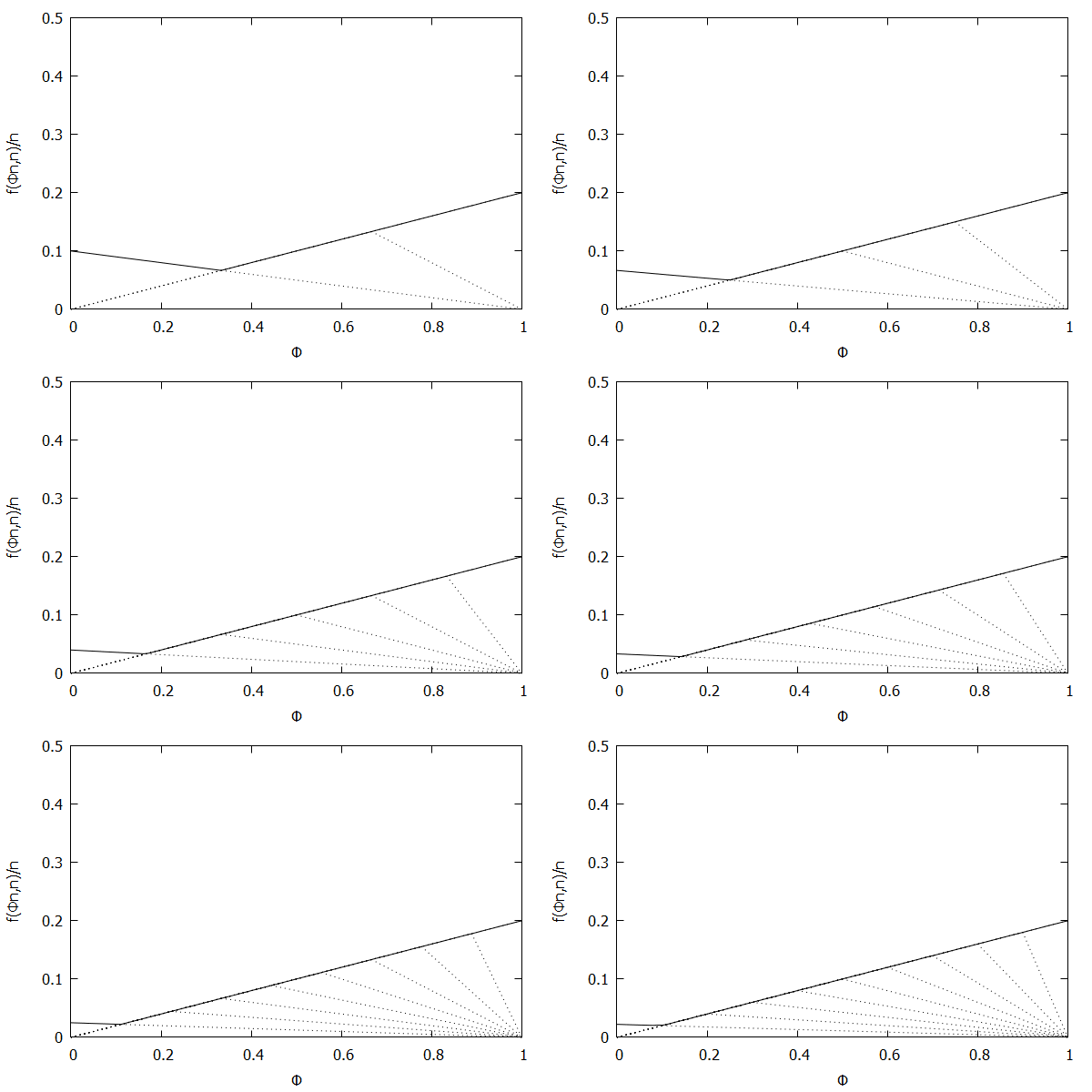
Now consider the low-biased quantile case, where we want lower quantiles to have higher precision than higher quantiles. In this case, the targeted quantile tuples set will become $\mathsf{T} = {(\frac{1}{n}, \frac{\epsilon}{n}), (\frac{2}{n}, \frac{2\epsilon}{n}), \ldots, (\frac{n-1}{n}, \frac{(n-1)\epsilon}{n}), (1, \epsilon)}$.

Given the above definition, below is a visualization of the error function $f(\phi n)/n)$ computed for $\epsilon$ = 0.1 as $n$ increases from 3 to 10:

Notice how the solid polyline allows less error at lower percentiles and is converging towards the line $f(\phi n, n)/n = 0.2\phi$, which exactly corresponds to the low-biased quantiles invariant function $f(r_i, n) = 2 \epsilon r_i$, as found in Definition 3 of [CKMS05].

High-Biased Quantiles Invariant Function

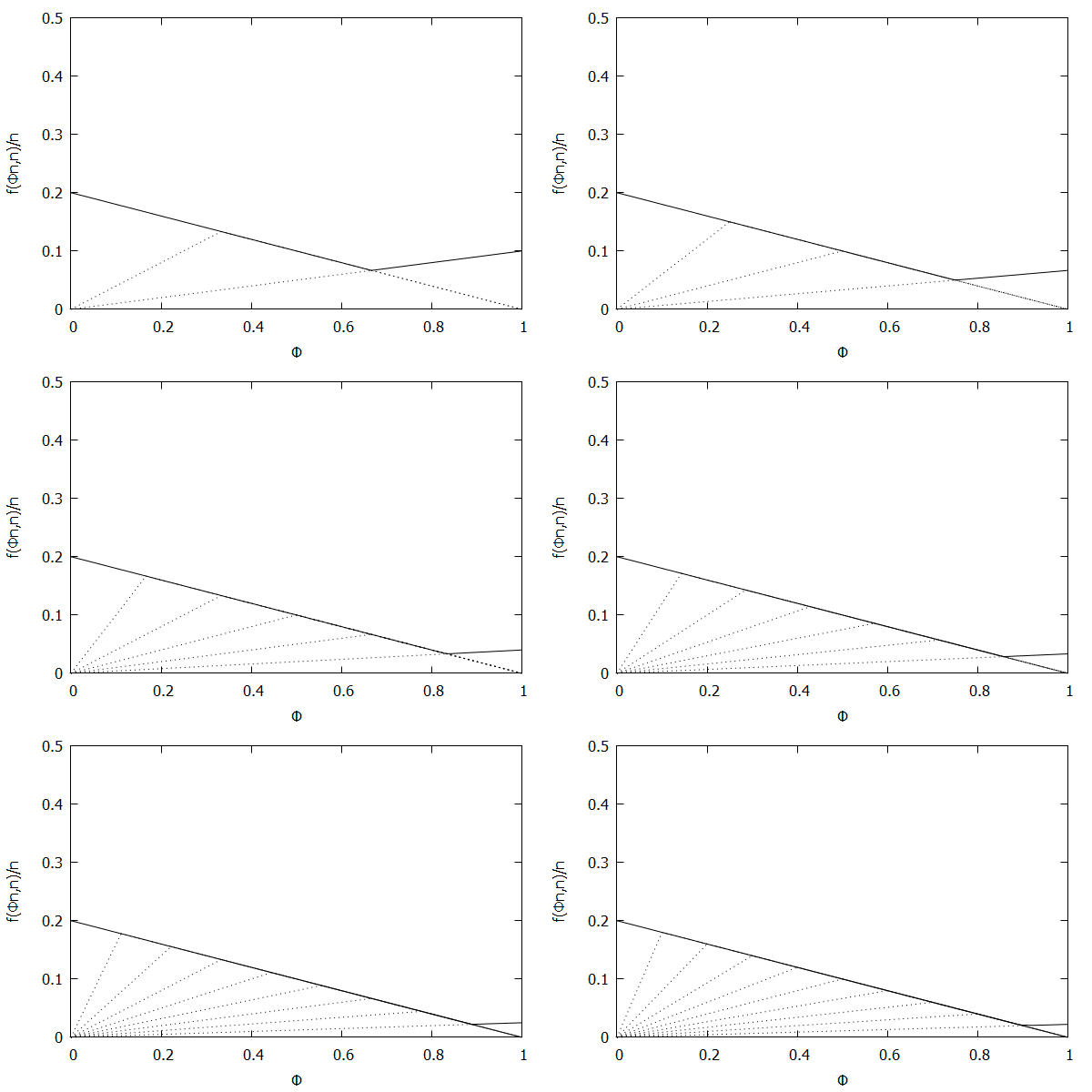
Now consider the high-biased quantile case, where we want higher quantiles to have higher precision than lower quantiles. In this case, the targeted quantile tuples set will become $\mathsf{T} = {(\frac{1}{n}, \epsilon), (\frac{2}{n}, \frac{(n-1)\epsilon}{n}), \ldots, (\frac{n-1}{n}, \frac{2\epsilon}{n}), (1, \frac{\epsilon}{n})}$.

Given the above definition, below is a visualization of the error function $f(\phi n)/n)$ computed for $\epsilon$ = 0.1 as $n$ increases from 3 to 10:

Notice how the solid polyline allows less error at higher percentiles and is converging towards the line $f(\phi n, n)/n = 0.2(1 – \phi)$, which corresponds to the high-biased quantiles invariant function $f(r_i, n) = 2 \epsilon (n – r_i)$ (not found in the [CKMS05] paper).

Availability in Streaming Percentiles Library

All four variants (uniform quantile, low-biased quantile, high-biased quantile, and targeted quantile) of the CKMS algorithm are available in my streaming percentiles library. Here’s an example of what it’s like to use:

1
2
3
4
5
6
7

#include <stmpct/ckms_hbq.hpp> // High-biased quantiles

ckms_hbq c(0.01);
for (int i = 0; i < 1000; ++i)
    c.insert(rand());
double p50 = c.quantile(0.5); // Approx. median
double p95 = c.quantile(0.95); // Approx. 95th percentile

Or, from JavaScript:

1
2
3
4
5
6

var sp = require('streamingPercentiles.v1.min.js');
var c = new sp.CKMS_HBQ(0.1);
for (var i = 0; i < 1000; ++i)
    c.insert(Math.random());
var p50 = c.quantile(0.5); // Approx. median
var p95 = c.quantile(0.95); // Approx. 95th percentile

For more information, visit the streaming percentiles library GitHub page.

References

• [GK01] M. Greenwald and S. Khanna. Space-efficient online computation of quantile summaries. In Proceedings of ACM SIGMOD, pages 58–66, 2001.
• [CKMS05] G. Cormode, F. Korn, S. Muthukrishnan and D. Srivastava. Effective Computation of Biased Quantiles over Data Streams. In Proceedings of the 21st International Conference on Data Engineering, pages 20-31, 2005.